Perform molecular dynamics simulations to study protein motion, validate binding stability, and analyze molecular behavior over time.

​

Overview

The Dynamo module provides an integrated environment for setting up, configuring, and running molecular dynamics simulations. Users can create custom simulation systems, define environmental conditions, adjust simulation parameters, and review system configurations before launching production runs. Molecular dynamics simulations help researchers evaluate protein flexibility, ligand stability, conformational changes, and molecular interactions under realistic physiological conditions.

​

Getting Started

​

Step 1: Open Dynamo

Navigate to Lab → Dynamo. The Dynamo home page displays existing simulations within a selected project and provides access to creating new simulation runs. Select the desired project from the project selector and click New Simulation.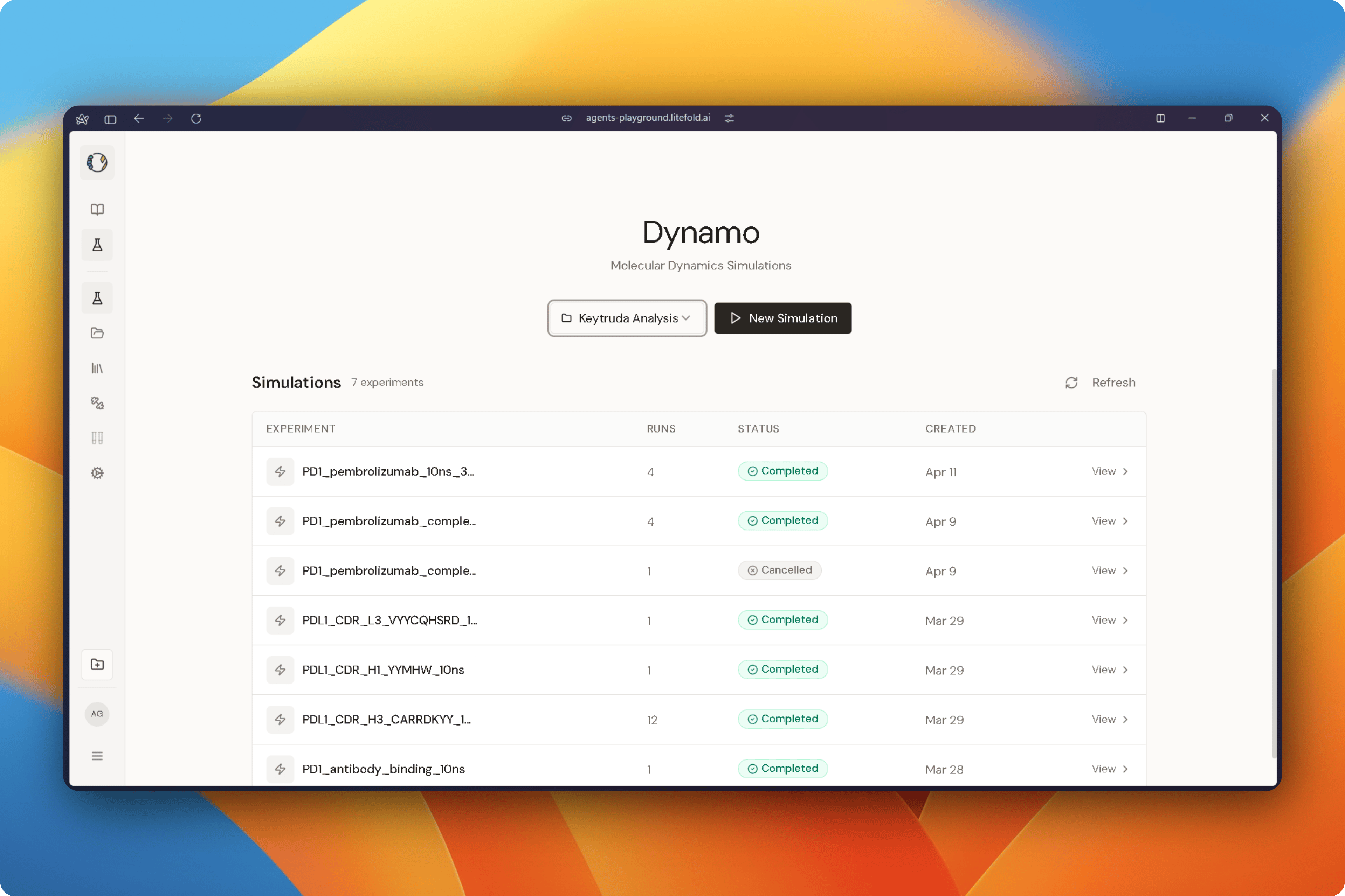

​

Creating a New Simulation

The simulation setup workflow consists of three stages:

1. System Setup
2. Parameters
3. Review

​

Step 1: System Setup

The System Setup page defines the molecular system that will be simulated.

​

Experiment Information

Provide a name for the simulation experiment. This name is used to organize simulation runs and distinguish them from other experiments within the project.

​

Membrane Simulation (Optional)

For membrane proteins, users can enable Membrane Simulation. When enabled, LiteFold automatically prepares a lipid bilayer environment around the protein using supported membrane force-field parameters.

​

System Molecules

The primary molecular components of the simulation are selected in this section. A simulation may contain:

• Protein
• Ligand / Cofactor
• Peptide
• DNA
• RNA

Multiple molecular components can be combined into a single simulation system when required. For each component, users select the corresponding structure file and force field.

​

Force Field Selection

For protein components, LiteFold allows users to select the force field used during simulation preparation and execution. Available force fields include:

• AMBER ff14SB — widely used protein force field optimized for biomolecular simulations.
• AMBER ff19SB — newer AMBER protein force field with improved backbone parameterization and protein conformational sampling.
• Espaloma — machine-learning-based force field generation framework designed to provide efficient molecular parameterization.

The selected force field determines how atomic interactions, bonded terms, and molecular energies are calculated throughout the simulation. For most protein simulations, AMBER ff14SB is recommended as the default choice, while AMBER ff19SB may provide improved performance for certain protein systems. Espaloma can be used when machine-learning-assisted parameterization is desired.

​

System Preview

As molecules are added, LiteFold generates a live system preview that allows users to verify the selected components before continuing.

​

Step 2: Configure Simulation Parameters

After defining the molecular system, click Next to open the Parameters page. This stage controls the physical and computational conditions used during simulation.

​

Simulation Type

LiteFold currently supports: Molecular Dynamics for classical atomistic simulations, Additional simulation engines may also be available depending on the deployment environment.

​

Simulation Duration

Defines the total simulation length. Examples include:

• 10 ns
• 50 ns
• 100 ns
• 200 ns

Longer simulations provide better conformational sampling but require additional computational resources.

​

Timestep

The timestep determines how frequently atomic positions are updated. Typical value: 4 fs Smaller timesteps improve stability while larger values improve computational speed.

​

Temperature

Simulation temperature is specified in Kelvin. Typical biological simulations use: 300 K which approximates physiological conditions.

​

Pressure

Pressure controls the simulation environment under NPT conditions. Typical value: 1 bar which approximates atmospheric pressure.

​

Solvation Settings

The solvation section defines the aqueous environment surrounding the system.

​

Water Model

LiteFold supports water models such as: TIP3P which is commonly used in biomolecular simulations.

​

pH

Defines the protonation environment used during preparation. Typical value: 7.2

​

Ionic Strength

Controls ion concentration within the solvent box. Typical value: 0.15 M which approximates physiological salt concentration.

​

Structure Preparation Options

​

Remove Heterogens

This option removes non-standard residues, crystallographic additives, and unwanted molecules during preparation. Removing heterogens helps generate a cleaner simulation system when only the primary molecular components are required.

​

Logging and Checkpoints

LiteFold allows users to define simulation output frequency.

​

Log Frequency

Determines how often simulation data is written to logs. Example: 250 steps

​

Checkpoint Frequency

Determines how often restart files are saved. Example: 25,000 steps Checkpoint files allow interrupted simulations to resume from the most recent saved state.

​

Advanced Settings

The Advanced section provides access to additional simulation controls, including specialized integrator settings, output configurations, and engine-specific parameters. These settings are generally intended for experienced users who require fine-grained control over simulation behavior.

​

System Preview

Throughout parameter configuration, LiteFold continuously updates the System Preview panel. The preview displays:

• Protein structure
• Ligands and cofactors
• Solvent environment
• Ions
• Additional molecular components

This allows users to verify the complete simulation system before launching the job.

​

Step 3: Review Simulation Configuration

The Review page summarizes the entire simulation setup.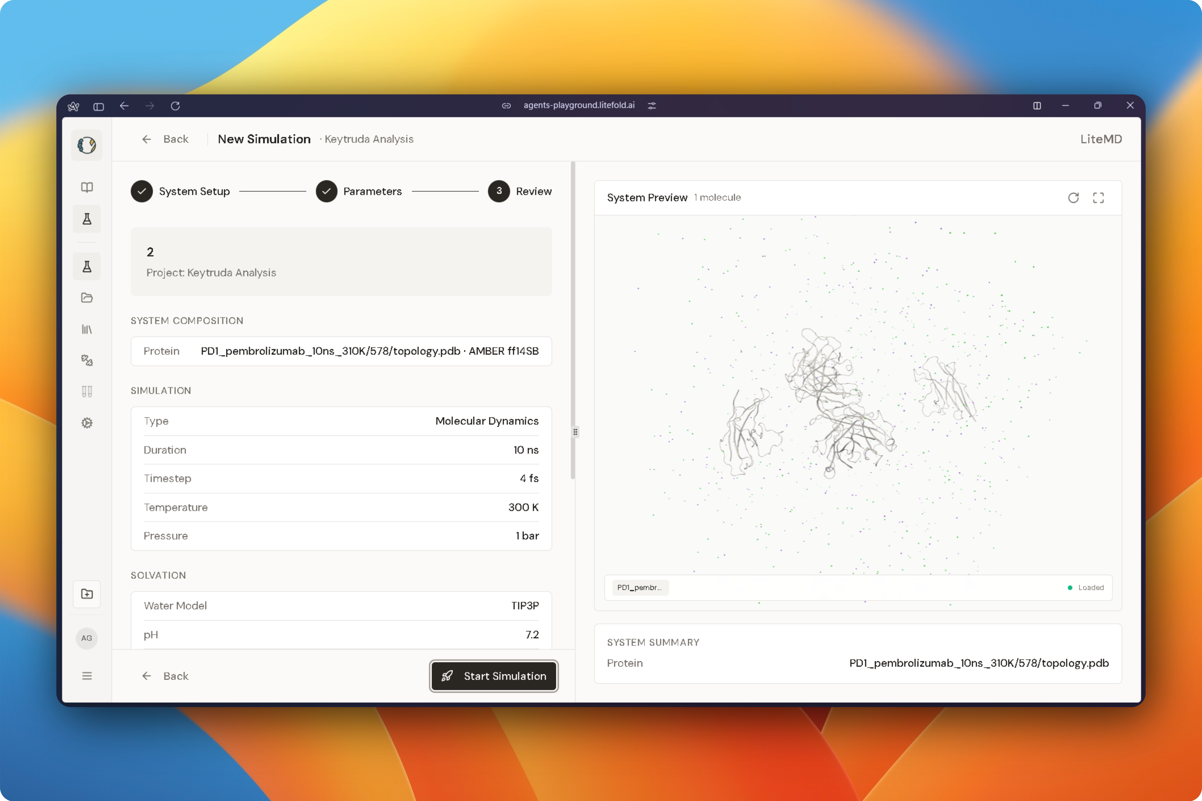

​

System Preview

A final visualization of the complete prepared system is shown alongside the configuration summary. This allows users to verify the setup before execution.

​

Launching the Simulation

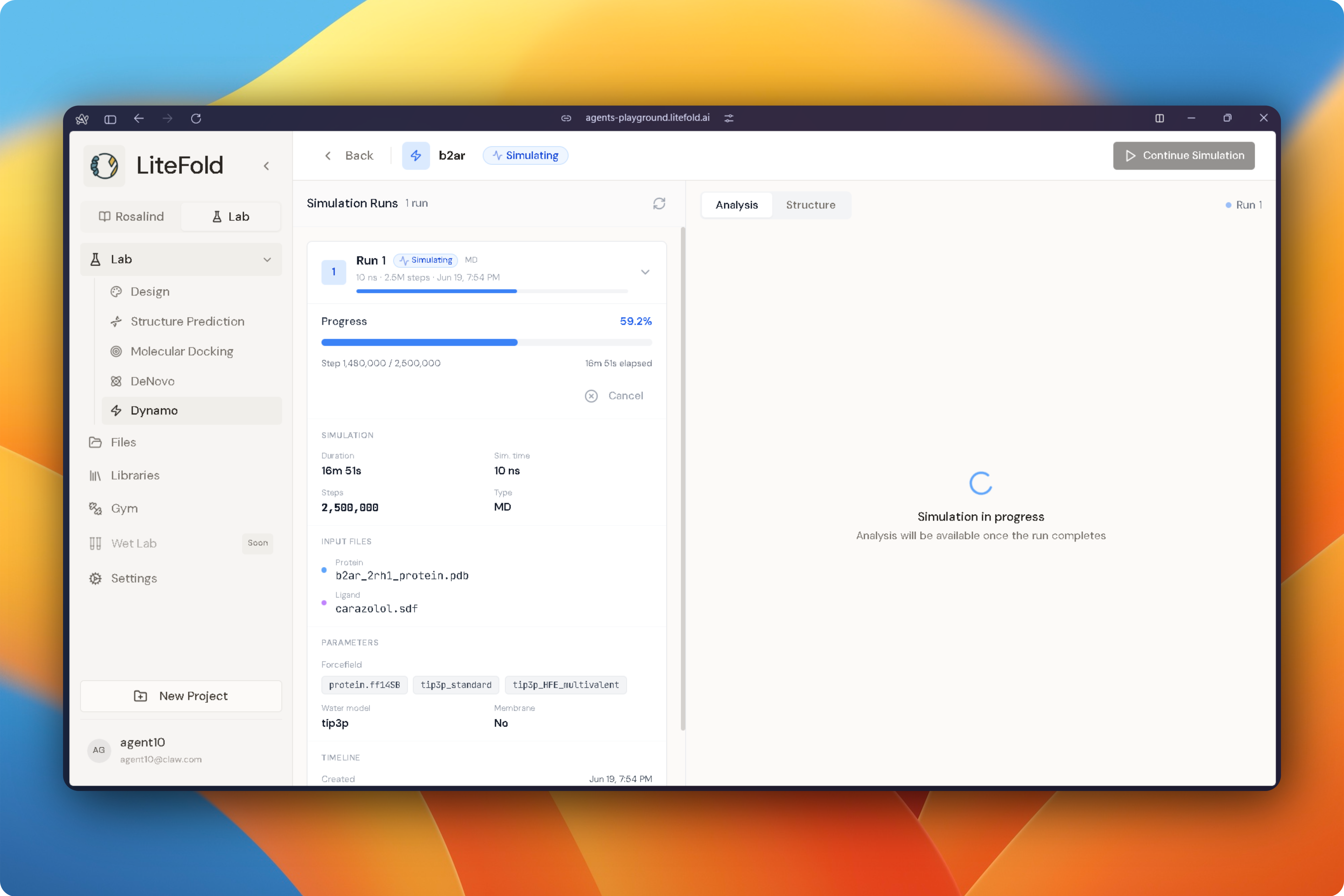
After confirming the configuration, click Start Simulation. LiteFold prepares the system, generates simulation files, and submits the job to the simulation engine. Simulation progress can then be monitored from the Dynamo dashboard.

​

Monitoring Simulation Progress

After a simulation is launched, LiteFold creates one or more simulation runs that can be monitored from the Dynamo results workspace. Each run displays detailed information about:

• Simulation duration
• Simulated time
• Total simulation steps
• Input structures
• Force fields used
• Water model configuration
• Membrane settings
• Timeline information
• Completion status

Users can review both active and completed simulation runs from the simulation dashboard.

​

Analysis Dashboard

The Analysis tab provides automated trajectory analysis generated directly from the simulation output. Rather than manually processing trajectory files, LiteFold calculates key structural and energetic metrics automatically. These analyses help determine whether the system remained stable throughout the simulation and identify important molecular behaviors.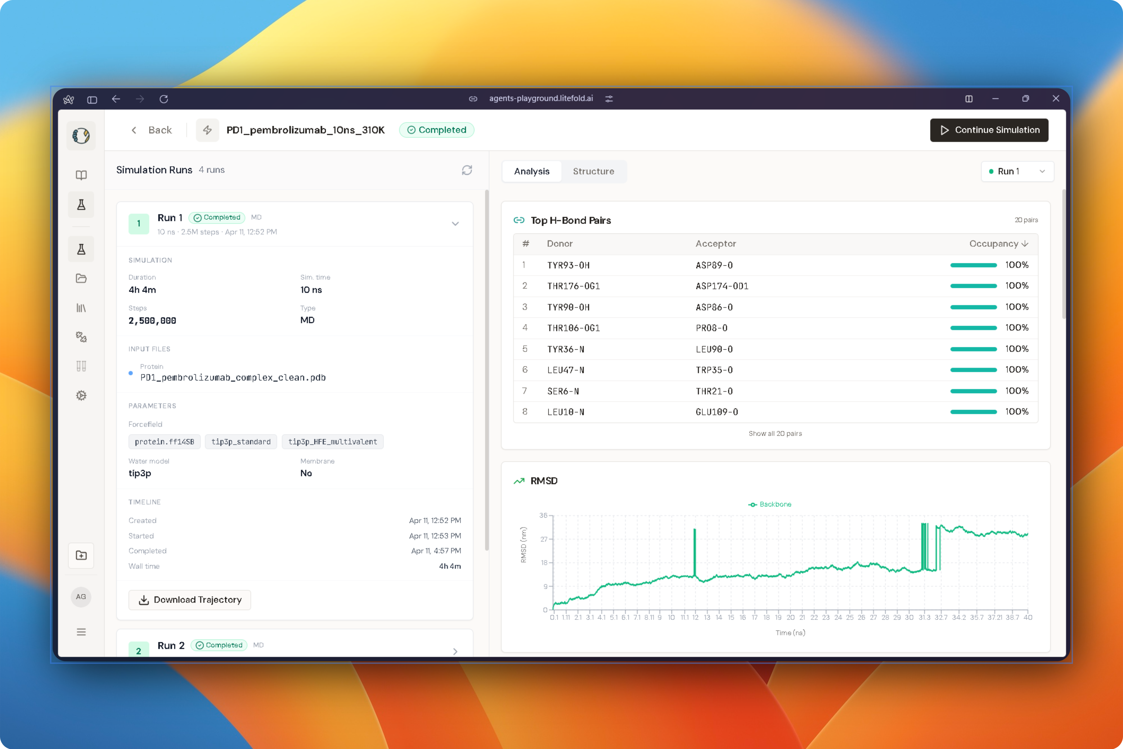

​

Hydrogen Bond Analysis

The Top H-Bond Pairs table identifies the most persistent hydrogen bonds observed during the simulation. For each interaction, LiteFold reports:

• Donor residue
• Acceptor residue
• Occupancy percentage

Occupancy indicates how frequently a hydrogen bond exists during the trajectory. A bond with high occupancy generally represents a stable interaction that contributes to structural integrity or ligand binding. dDA≤3.5 A˚ and The hydrogen bond angle criterion is defined as: $\theta_{D-H-A} \geq 120^\circ$ Where:

• D = Donor atom
• H = Hydrogen atom
• A = Acceptor atom
• θ = Bond angle formed by D-H-A

Larger bond angles generally indicate stronger and more favorable hydrogen-bond interactions.

​

Hydrogen Bond Occupancy

The percentage of simulation frames containing a given hydrogen bond is calculated as: $$\text{Occupancy} = \frac{N_{HB}}{N_{total}} \times 100$$ Where:

• $N_{HB}$ = Number of frames containing the hydrogen bond
• $N_{total}$ = Total number of trajectory frames

Higher occupancy values indicate that the hydrogen bond is maintained for a larger portion of the simulation, suggesting greater interaction stability.

​

RMSD Analysis

Root Mean Square Deviation (RMSD) measures how much the structure changes relative to its starting conformation during the simulation. The RMSD plot allows users to evaluate:

• Structural stability
• Convergence behavior
• Major conformational shifts
• Equilibration quality

The Root Mean Square Deviation (RMSD) is calculated as: $$RMSD(t) = \sqrt{\frac{1}{N}\sum_{i=1}^{N}\left|r_i(t)-r_i^{ref}\right|^2}$$ Where:

• $N$ = Number of atoms
• $r_i(t)$ = Position of atom $i$ at time $t$
• $r_i^{ref}$ = Reference position of atom $i$

​

Interpretation

• Low RMSD → stable structure
• High RMSD → significant conformational change

​

RMSF Analysis

Root Mean Square Fluctuation (RMSF) measures residue-level flexibility throughout the trajectory. The RMSF plot helps identify:

• Flexible loops
• Stable structural cores
• Dynamic regions
• Mutation-sensitive areas

The Root Mean Square Fluctuation (RMSF) is calculated as: $$RMSF(i) = \sqrt{\frac{1}{T}\sum_{t=1}^{T}\left|r_i(t)-\langle r_i \rangle\right|^2}$$ Where:

• $T$ = Total simulation frames
• $r_i(t)$ = Position of residue $i$ at time $t$
• $\langle r_i \rangle$ = Average position of residue $i$

Interpretation:

• Low RMSF values indicate relatively rigid regions of the structure.
• High RMSF values indicate flexible loops or highly mobile domains.

​

Potential Energy Analysis

LiteFold automatically tracks system potential energy throughout the simulation. Potential energy plots are useful for evaluating:

• System equilibration
• Energy stability
• Simulation quality
• Unexpected energetic fluctuations

The total potential energy of the system is calculated as: $$E_{total} = E_{bond} + E_{angle} + E_{dihedral} + E_{vdW} + E_{electrostatic}$$ Where:

• $E_{bond}$ = Bond stretching energy
• $E_{angle}$ = Bond angle bending energy
• $E_{dihedral}$ = Torsional (dihedral) energy
• $E_{vdW}$ = Van der Waals interaction energy
• $E_{electrostatic}$ = Electrostatic interaction energy

Stable energy profiles generally indicate that the system has reached equilibrium and remains thermodynamically stable throughout the simulation.

​

Structure Visualization

The Structure tab provides an interactive molecular viewer for examining simulation structures. Users can inspect:

• Protein conformations
• Ligand positions
• Molecular interactions
• Structural changes observed during simulation

This allows visual validation of behaviors observed in the analytical plots.

​

Checkpoints and Continuing Simulations

During execution, LiteFold periodically creates checkpoint files according to the checkpoint frequency defined during simulation setup. Checkpoint files store the current state of the simulation, including atomic coordinates, velocities, and simulation progress. These checkpoints serve two purposes. First, they protect against data loss by allowing interrupted simulations to resume from the most recent saved state. Second, they allow users to extend completed simulations without starting over from the beginning.

​

Continue Simulation

LiteFold allows completed or partially completed simulations to be extended using the Continue Simulation feature. When a simulation is resumed, the platform automatically loads the most recent checkpoint and continues the run from the exact state where it previously stopped. This preserves all trajectory data, system coordinates, velocities, and simulation history generated during the earlier run. Extending a simulation is useful when additional sampling is needed, when structural metrics such as RMSD have not yet stabilized, or when longer trajectories are required for more reliable analysis. Researchers may also choose to continue a simulation after observing interesting conformational changes that warrant further investigation. For example, a simulation initially run for 10 ns can be extended to 50 ns, 100 ns, or longer without restarting the calculation. This approach saves computational time and enables continuous analysis of the same molecular system across multiple simulation stages.

​

Downloading Trajectories

LiteFold allows users to download simulation trajectories directly from the results page. Trajectory downloads typically include:

• Atomic coordinates
• System topology
• Simulation metadata
• Analysis-ready trajectory files

Downloaded trajectories can be further analyzed using external molecular dynamics software such as VMD, PyMOL, GROMACS tools, MDTraj, or MDAnalysis.

​

Interpreting Simulation Stability

A simulation is generally considered well behaved when:

• RMSD reaches a stable plateau
• Potential energy remains stable
• Key hydrogen bonds remain persistent
• RMSF values are consistent with expected protein flexibility

When significant structural drift or unstable energy behavior is observed, longer simulations or additional replicates may be required before drawing conclusions.

​

Best Practices

Use properly prepared structures before starting simulations. Verify that all molecular components are correctly assigned and review the system preview carefully. For protein-ligand systems, ensure the ligand occupies the intended binding site before launching production runs. For important studies, running multiple independent simulations can help assess reproducibility and improve confidence in observed molecular behavior.

​

Next Steps

After a simulation is completed, the generated trajectories and structural data can be used for:

• RMSD analysis
• RMSF analysis
• Hydrogen-bond analysis
• Contact analysis
• Binding stability assessment
• Free-energy calculations
• Lead optimization studies
• Structure-based drug discovery workflows

This enables users to move from static structures to a dynamic understanding of molecular behavior under realistic biological conditions.

​

Next Steps

​

Next Steps